
The authors examine GNSS performance on 27,500 kilometers (17,000 miles) of North American highways to better understand the automotive positioning needs it meets today and what might be possible in the near future with wide area GNSS correction services and multi-frequency receivers.
By Tyler G. R. Reid, Nahid Pervez, Umair Ibrahim, Sarah E. Houts, Gaurav Pandey, Naveen K. R. Alla, and Andy Hsia.
Authors from Xona Space Systems, Ford Motor Company, and Ford Autonomous Vehicles, LLC.
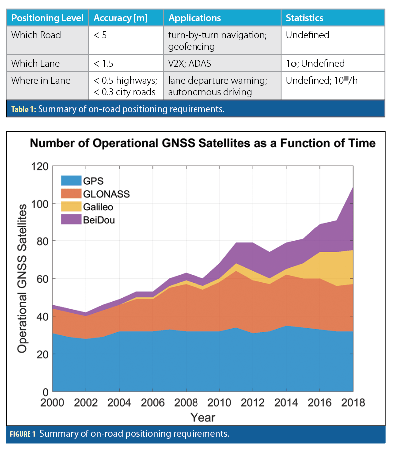
Vehicle location information assumes ever-increasing importance for Advanced Driver Assistance Systems (ADAS), connectivity (V2X), and Autonomous Driving (AD) features. Some features, such as turn-by-turn navigation instructions, provide convenience, where others, such as lane departure warning and lane-keeping, are safety-critical. New applications are driving more stringent localization requirements for position information at the level of which road, which lane, or where in the lane. While strict requirements on these categories have yet to be defined, Table 1 provides some data points.
Road standards in the United States call for highway lanes to be 3.6 meters wide and local/city lanes to be at least 2.7 meters wide. Hence, which-road positioning is generally taken as slightly better than two lane widths, as this is the typical width of most two-way roads. Some applications that require this level of positioning are turn-by-turn navigation and geofencing. For example, Cadillac’s Super Cruise level 2 self-driving feature is currently geofenced to limited access divided highways. Super Cruise utilizes precision Light Detection and Ranging (LiDAR) maps of select US and Canadian divided highways from Ushr in conjunction with GNSS correction services from Trimble’s RTX to achieve high confidence geofencing of the feature. This and other SAE level 2 self-driving features represent partial automation, where the human driver is responsible for monitoring the scene and the system is responsible for some dynamic driving tasks including steering, propulsion, and braking. The human driver must be ready to take over dynamic driving tasks immediately when the driver determines the system is incapable.
For which-lane positioning, most reasonably trafficked US roads are built with 3+ meter lane widths; better than half of this number, or 1.5 meters, is generally accepted as lane determination. The National Highway Safety Administration (NHTSA) has, as part of its Federal Motor Vehicle Safety Standards in Vehicle to Vehicle (V2V) Communications, determined that position must be reported to an accuracy of 1.5 meters (1σ or 68%) as this is tentatively believed to provide lane-level information for safety applications.
The most stringent positioning is that needed for maintaining the vehicle within its lane. This requirement is a combination of road geometry (width and curvature) along with vehicle dimensions. The small spaces between vehicle edges and the painted lines on the road are the required position protection level to maintain the vehicle within its lane. For passenger vehicles in the US, highway road geometry requires <0.5 meters lateral positioning, while local/city road geometry require <0.3 meters. For fully autonomous operation, these protection levels must be maintained to an integrity risk of 10-8 failures/hour of operation. This is equivalent to 99.999999% certainty in position.
Many localization technologies have been proposed to meet these needs. Relative navigation sensors based on LiDAR, computer vision, and others work by localizing to an a-priori map. This functions well in feature-rich urban environments but can degrade in sparse highway settings. Qualitatively, positioning based on GNSS is complementary, where a lack of features is typically synonymous with open skies and favorable satellite visibility. This article focuses on the state of GNSS on predominantly highways in North America in 2018 and attempts to answer where it fits within ADAS, V2X, and AD today and in the near future.
Since 2010, the number of navigation satellites available has more than tripled, moving from GPS-only (USA) to the inclusion of a rebooted GLONASS (Russia) constellation in 2011 and now nearly completed Galileo (Europe) and BeiDou (China) constellations. There are now more than 100 operational navigation satellites in orbit. For the user, this implies a jump from 10 to 30+ satellites in view and has significant implications for on-road GNSS availability.
Multi-constellation is just one of the advances coming to the automotive domain; the others are multi-frequency and widespread corrections services. The use of these technologies is not new to the automotive domain. Survey grade GNSS receivers coupled with a tactical grade Inertial Measurement Unit (IMU) and correction services are often used in testing, validation, and research. Traditionally such systems came at a high cost, however, we are now in a state of transition from specialized to volume markets and many technologies are rapidly maturing in large-scale efforts in production to meet the demand for decimeter location. On the GNSS side, multi-frequency mass-market receivers are already here. Real-Time Kinematic (RTK) and Precise Point Positioning (PPP) correction services are becoming more capable and more available, giving rise to sub-decimeter convergence in a matter of minutes or even seconds.
Here, we examine the performance of multi-constellation GNSS and corrections on 27,500 km of U.S. and Canadian highways. A representative production-grade automotive multi-constellation GNSS L1-only receiver was driven in tandem with a survey-grade GNSS receiver used as ground truth. Furthermore, the ground truth was an inertial navigation system which combines two multi-frequency (L1+L2) GNSS receivers with a tactical-grade micro-electro-mechanical systems (MEMS) inertial measurement unit (IMU). The two-receiver configuration is used to calibrate heading/attitude and the IMU. The ground-truth system utilized networked RTK corrections delivered in real time via a cellular link.
The analysis examines GNSS accuracy, availability, and continuity. Position accuracy of the representative production-grade automotive GNSS was determined through direct comparison with the ground-truth system. Accuracy of the RTK-enabled ground truth was estimated from the position uncertainty output from the combined INS solution. Availability of satellite visibility and geometry (dilution of precision) was examined for both the survey-grade and production-grade units. Availability of RTK positioning and corrections is also assessed. All accuracy and availability metrics are compared statistically and geospatially on a map. The probability of continuity loss over timescales associated with critical automotive maneuvers is developed for metrics on satellite visibility, geometry, and RTK positioning. Statistics on outage times are also presented. These performance indicators inform the potential role of GNSS as one of several positioning sensors in ADAS, V2X and AD.
Methodology
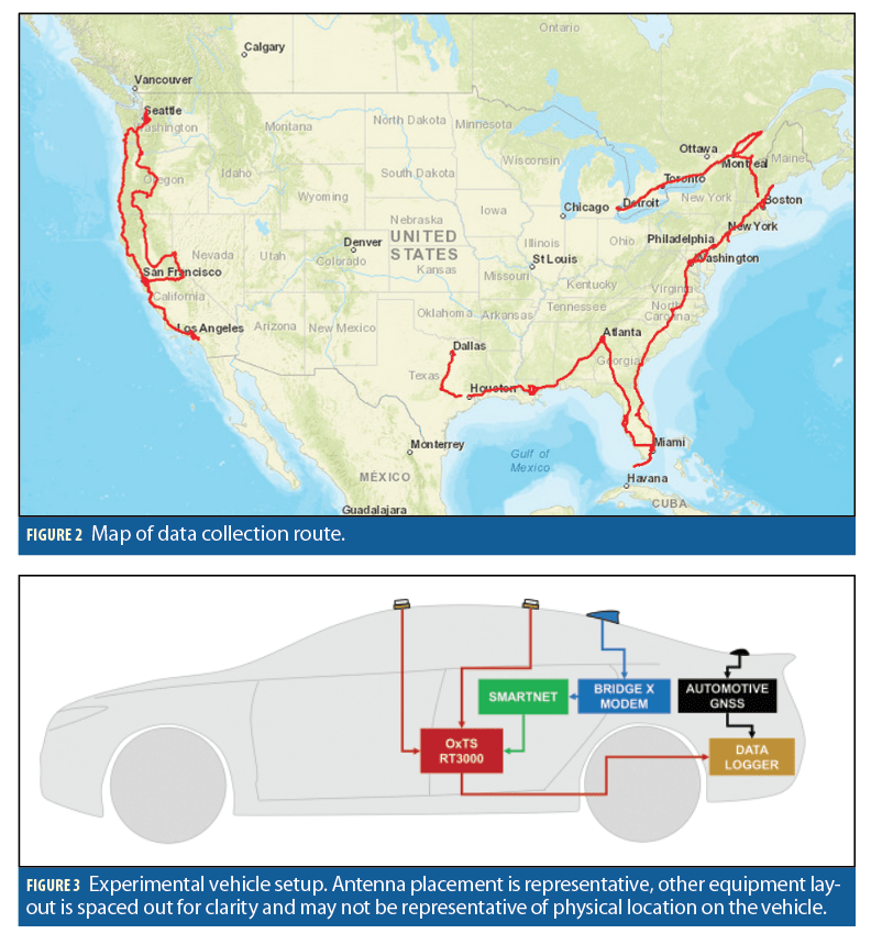
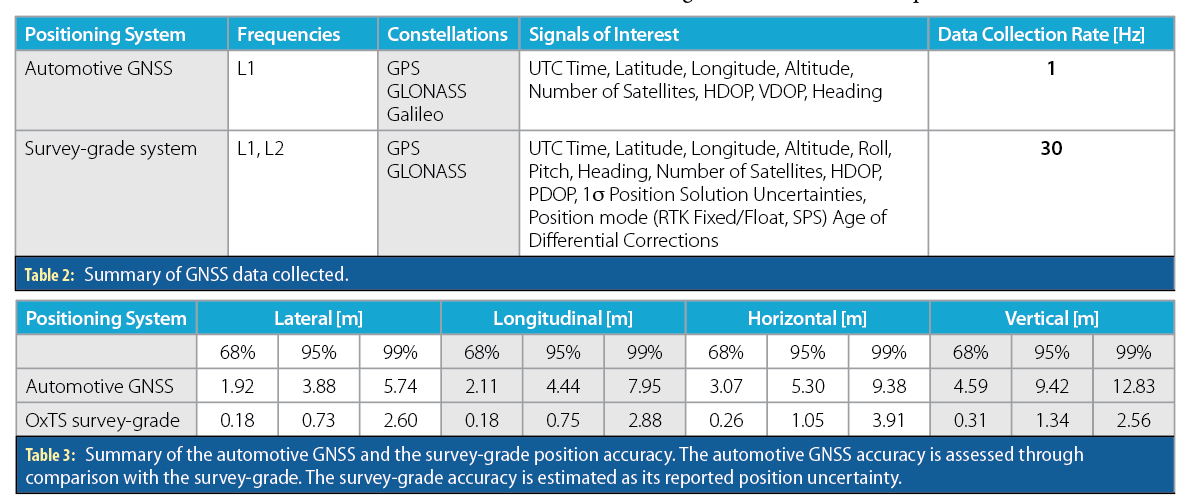
The dataset was driven in mid 2018, primarily targeting the population centers of the east and west coasts of the U.S. and Canada on the route shown in Figure 2. Two separate vehicles were used in the data collection, one on each coast. The experiment design and hardware setup were largely the same on both vehicles. A high-level summary of the data collection vehicles and GNSS data collected is given in Figure 3and Table 2, respectively.
A total of 27,500 kilometers was driven, representing 355 hours (~15 full days) of data. This was largely highway driving, though some of the route did pass through major urban centers. To put this in perspective, the U.S. National Highway System (NHS) consists of approximately 350,000 kilometers (220,000 miles) of road. Hence, the data shown here represents roughly 8% of the NHS. Although NHS accounts for only 5% of total road mileage in the United States, it carried 55% of the 1.64 trillion miles travelled in the U.S. in 2015.
Two separate GNSS systems were used in data collection, one representative of that used in production vehicles today and the other a survey-grade system to act as a reference or ground truth. The production-oriented GNSS was automotive grade, multi-constellation capable (GPS + GLONASS + Galileo), and utilized the L1 frequency only. The survey-grade system combined two survey-grade GNSS receivers with an IMU to provide the ability to coast through reasonable GNSS outages. The units used in this experiment were GPS + GLONASS and capable of tracking both the L1 and L2 frequencies. The MEMS IMU is tactical grade with a gyro bias stability of 2 degrees/hour. The two GNSS receivers are used to constantly calibrate the attitude of the IMU, primarily to provide heading.
Networked RTK corrections were also used in this experiment. Cellular connectivity was available on the vehicle and corrections were delivered via a modem and networked RTK corrections were provided by commercial network, where coverage was available along the entire data collection route. See Table 2 for summary of data collected.
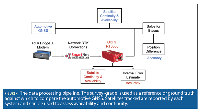
Using internal tools, time synchronization was achieved between the automotive grade GNSS and survey-grade. Aggregate statistics were produced on satellite visibility and geometry to establish availability and continuity. The same was done on parameters related to RTK positioning. Assessment of position accuracy requires a more detailed examination. The production GNSS was compared to what was considered ground truth, the INS solution from the survey-grade system; the latter is itself not without flaws, hence only highly confident position solutions were used in the comparison. The mathematics of how to compare these systems and remove systematic biases is described an appendix available from the authors. These biases are removed as it is assumed they can be reasonably calibrated out as will be described in the next section. The process is summarized in Figure 4.
Accuracy
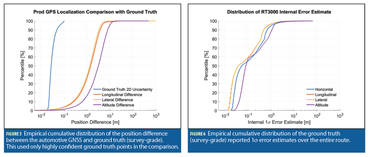
The production-grade automotive GNSS position error is assessed by direct comparison to the survey-grade which is considered ground truth using the methodology described in the appendix. To add reliability to this assertion, only highly confident survey-grade INS position solution points were used in the comparison. These were taken as having a horizontal position uncertainty of σH< 10 centimeters, a parameter output from the survey-grade itself. These were primarily the RTK-fixed positions of the survey-grade and hence the most reliable. As will be shown, this is taking points that are at least an order of magnitude more accurate than the automotive GNSS under investigation. The error distribution of the survey-grade itself was estimated from this reported uncertainty output σH.
The cumulative position error distributions for the automotive GNSS and survey-grade are given in Figures 5 and 6, respectively, and a high-level summary is given in Table 3. Many factors contribute to the performance in lateral and longitudinal accuracy including the vehicle-relative location of obstructions due to buildings, trees, signs, and other vehicles, affecting satellite geometry and multipath. Results indicate longitudinal accuracy to be slightly worse compared to lateral for the automotive GNSS. This result could also be indicative of delays in the system where at typical highway speeds, the 68th percentile difference of 20 centimeters between lateral and longitudinal could be the manifestation of a time mismatch of 5 milliseconds, not unreasonable for vehicle Controller Area Network (CAN) signals.
The survey-grade cumulative position error distribution in Figure 6 shows no significant difference between the lateral and longitudinal position errors. Closer examination shows that this distribution has three distinct regimes corresponding to the quality of the different positioning modes. In the centimeter regime, there are the ‘RTK fixed’ solutions, where the system is successful in carrier-phase integer ambiguity resolution. In the decimeter regime, there are the ‘RTK float’ solutions, where only floating-point estimates of the carrier phase integer ambiguities are available. The final meter-level regime is standard code-phase positioning where either RTK corrections were unavailable or obstructions disrupted carrier phase tracking. Furthermore, this shows that only 55% of positions were estimated as better than 10 centimeters horizontal. These represent predominantly RTK fixed solutions and were those used in the comparison with the automotive GNSS. Hence, the full distribution shown for the RT represents both good and bad GNSS conditions. In contrast, the automotive GNSS error is estimated in places where the survey-grade showed good performance and was likely in favorable GNSS environments.
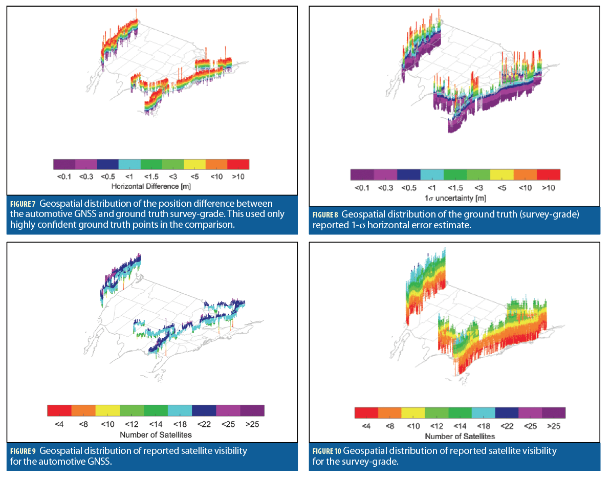
The geospatial distribution of horizontal position errors for the automotive GNSS and survey-grade are given in Figures 7 and 8, respectively. This shows the spatial uniformity of the errors. Though there are some spikes in Figure 7 with the automotive GNSS, these locations correspond to areas that pass through major urban centers and hence urban canyons with poor satellite visibility. In these environments, poor geometry is further compounded by the presence of multipath and non-line-of-sight (NLOS) signals.
Availability
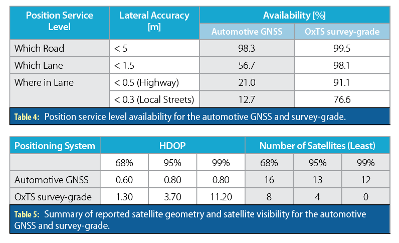
Table 4 shows position service level availability broken down by which-road, which-lane, and where-in-lane performance. This indicates that the automotive GNSS is capable of road determination 98.3% of the time, though it is less suitable for lane-level or where-in-lane applications at 56.7% and 21.0%, respectively. By comparison, the survey-grade is capable of road determination 99.5% of the time, lane determination at 98.1%, and where-in-lane highway applications at 91.1%. At the points where the automotive GNSS was evaluated, the survey-grade was confident at <10 cm, hence having 100% availability in all of the categories listed at these epochs. Something not considered here is the error budget allocation needed in the global accuracy of the map in these use cases. Ultimately, if the desire is to perform lane-determination or lane-keeping through a combination of GNSS with a lane-level map, then the global uncertainty of the map and the uncertainty of the GNSS position stack up. This will ultimately lead to more stringent requirements on GNSS; however, we feel these numbers are a good starting point.
At the root of positioning performance is the availability of satellites both in numbers and spatial diversity (i.e. geometry). In this context, this is a combined measure of satellites available above the horizon and environmental factors causing satellite obstructions. A summary of these results is given in Table 5.
This shows the 68th percentile number of satellites available for the automotive GNSS to be 16 with GPS + GLONASS + Galileo compared to 8 with the GPS + GLONASS survey-grade. The 99th percentile shows an even starker difference at 12 and 0, respectively. In part, this signifies the increased availability from a third constellation, adding approximately 8 more satellites above the horizon. However, the full story is given by the geospatial distribution of satellite visibility for the automotive GNSS and survey-grade shown in Figures 9 and 10. This shows a difference in how satellite visibility is reported between these two receivers. The survey-grade is constantly dropping down to zero as a result of overpasses and other occlusions. The automotive GNSS does not show this behavior but instead gives more of what appears to be an average sense of satellites above the horizon rather than satellites instantaneously tracked. The survey-grade shows spatial uniformity in that good and bad satellite visibility is seemingly evenly dispersed. The automotive GNSS has low points only in a handful of places which correspond to major urban centers with prolonged satellite outages.
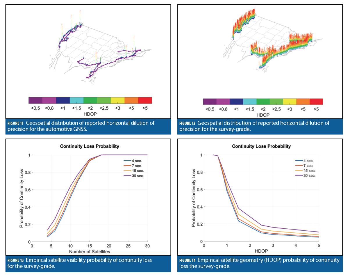
Satellite geometry as described by Horizontal Dilution of Precision (HDOP) is also summarized in Table 5.Similarly, the geospatial distributions are given in Figures 11 and 12. These again show spatial uniformity. Though there are some spikes with the automotive GNSS, these locations again correspond to areas that pass through major urban centers and hence urban canyons, showing a strong correlation between satellites in view and HDOP. Another observation is that the West Coast generally has slightly worse HDOP overall. This characteristic could be explained by the generally more mountainous terrain, which can introduce a higher elevation angle mask.
Continuity and Outage Times
We focus on satellite continuity in terms of number and spatial diversity. The emphasis will be on the survey-grade as its data was available at a high rate (>30 Hz) compared to the automotive GNSS (1 Hz), this represents GPS + GLONASS.
In critical aviation maneuvers, the timescale of interest for continuity is 15 seconds. The allocated continuity loss risk over this time period is 8×10⁻⁶ for both precision approach and instrument landing. Assumptions with this allotment are that GNSS is the primary navigation signal and that the sky is unobstructed and hence loss in continuity is coming from the signal in space.
In the automotive domain, the timescales of interest correspond to the duration of critical maneuvers such as lane changes, overtaking, and for highly automated systems, driver handover time. The duration of lane changes has been shown to typically be 4 seconds but could take up to 13 seconds in some conditions. Overtaking maneuvers on two-lane highways are typically 7 seconds but could take up to 17 seconds. Automated-to0-manual driving handover takes between 2.8 and 23.8 seconds, assuming the driver is involved in a secondary task such as reading before regaining control.
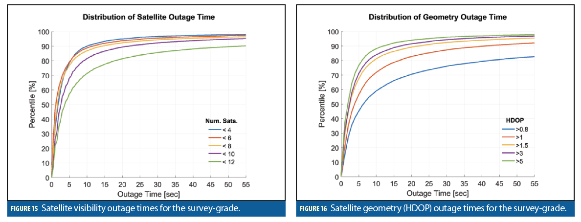
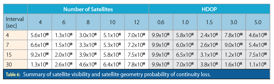
Based on these maneuvers, we examined the probability of continuity loss in 4, 7, 15, and 30 second intervals (Table 6). Figures 13 and 14 give a more detailed look at satellite visibility and HDOP. These show the spread of continuity loss to be small over the time intervals of interest for a given number of satellites or level of HDOP. Even for the shortest interval of 4 seconds, probabilities of continuity loss are on the order of 10-1, nearly 5 orders of magnitude worse than numbers assumed in critical aviation maneuvers. These directly impact the continuity of the position solution.
Figures 15 and 16 give the cumulative distribution of outage times for satellite visibility and HDOP.
RTK Performance
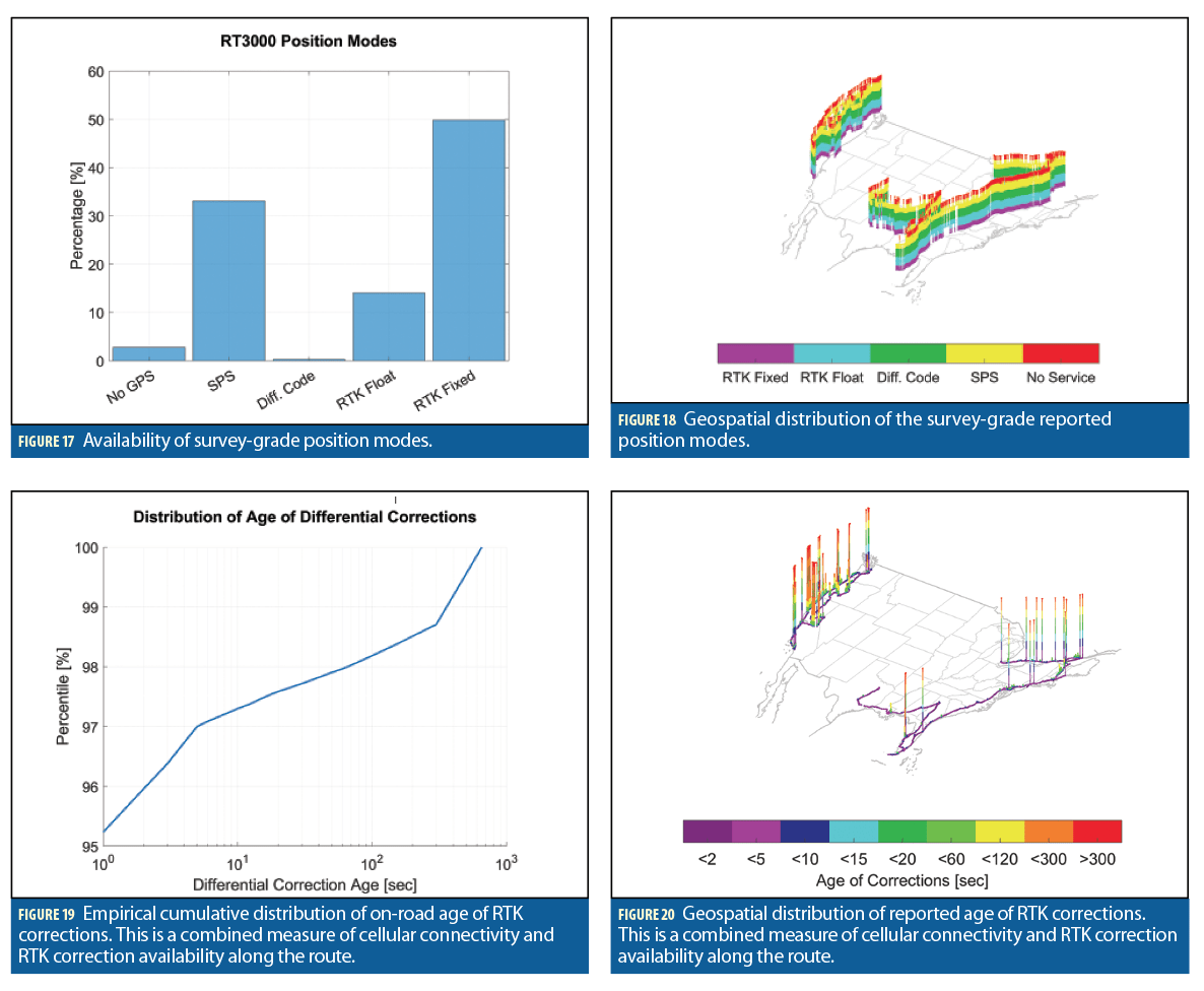
Table 7 shows a summary of position mode and networked RTK correction availability. Position mode availability is a combined measure of environmental factors which cause obstructions to satellites and availability of RTK corrections delivered in real time over the cellular network. Carrier-phase integer ambiguity resolution (RTK fixed) is achieved in nearly 50% of positions. These are the centimeter-level positions in the distribution shown in Figure 6. Carrier-phase floating point solutions (RTK float) are achieved in 14% of cases. Majority of other data points were reported as standard code-phase positioning (33%) with very few being differential code-phase (<1%). The latter likely converged quickly to a floating-point carrier-phase solution. Figure 17 summarizes position mode availability.
Figure 18 gives the geospatial distribution of position mode. Position mode is not continuous but instead constantly dropping from RTK-fixed to standard code-phase positioning (SPS) or even to no position fix. This is a result of the continuity of satellite visibility and geometry earlier along with availability of RTK corrections.
Table 7 summarizes the age of RTK corrections used by the receiver; stale corrections would only be used if new ones were unavailable. ‘Stale’ in the context of networked RTK is typically taken as older than 10 to 15 seconds due to the temporal decorrelation of GNSS satellite, clock, and atmospheric errors between the base station and rover receiver (vehicle). Since corrections were delivered in real time, availability is predominantly a measure of cellular coverage along the route. Nearly 96% of corrections are less than 2 seconds old, which is considered to be low latency and hence good performance. In 97% of cases, new corrections could take up to 10 seconds to arrive. In the remaining 3% of cases, corrections could be several minutes old due to extended cellular network outages and be of limited value. Figure 19 shows the cumulative distribution of correction age, and Figure 20 the geospatial distribution of correction age. Spikes occur mostly in rural areas with poor cellular coverage.
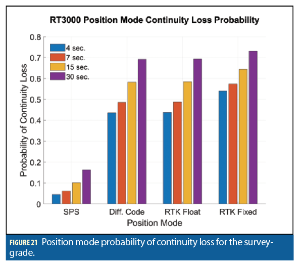
Table 8 and Figure 21 depict the probability of continuity loss of RTK and other position modes. Continuity is on the same order as that for satellite visibility and geometry discussed earlier. The ranking of solution fragility is inversely related to accuracy following the order of RTK fixed, RTK float, differential code-phase, and SPS with RTK fixed being most accurate and most transient. This is expected due to the increased difficulty of tracking carrier phase compared to code phase used in SPS positioning. Like satellite visibility and dilution of precision, these are on the order of 10-1, a stark difference from the 10-6 numbers assumed in critical aviation maneuvers. This is one challenge facing development of high-integrity GNSS positioning systems on the road.
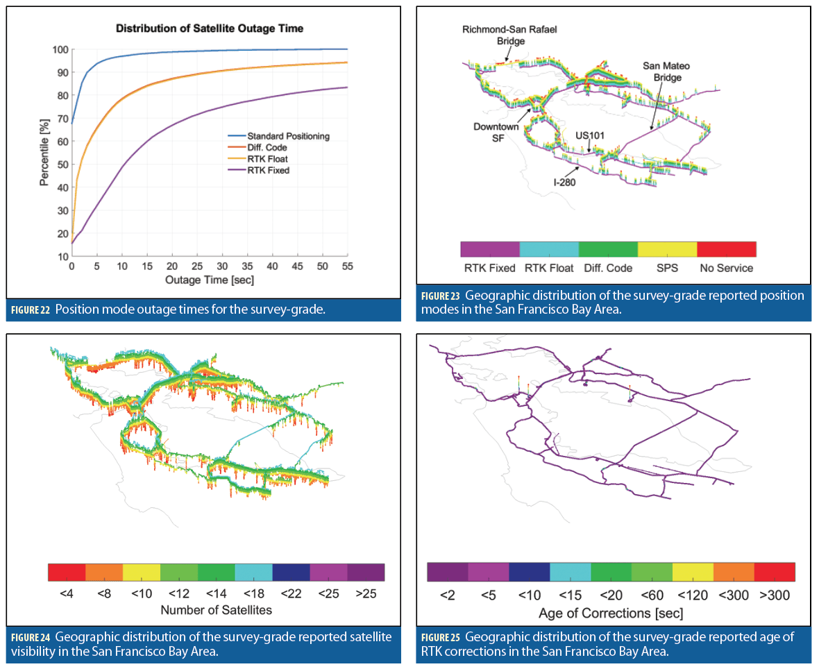
Figure 22 shows typical outage times. Median RTK fixed outages are 11 seconds compared to float solutions at 2 seconds. However, in 95% of cases, outages for RTK fixed and float can be longer than a minute, compared to standard code phase positioning at <7 seconds. RTK outages can be much longer than timescales of critical maneuvers considered.

Case Study: San Francisco Bay Area
To show these factors combined in defining GNSS performance, consider the example of the San Francisco Bay Area in California. Figure 23 shows the position mode map where it is clear that open highways such as the I-280 and US101 have RTK fixed performance with dropouts corresponding to overpasses. The San Mateo Bridge is in open sky and also has very good performance. By comparison, the Richmond-San Rafael Bridge shows poor performance as this was driven eastbound on the lower deck. Downtown San Francisco shows intermittent performance with many dropouts due to obstructions from tall buildings. Figure 24 shows a strong correlation with these events and satellite dropouts. Figure 25 shows that the RTK correction latency was less of a factor, indicating an adequate cellular data connection with the exception of three data points.
Though bulk measures of accuracy, availability, and continuity here are useful for assessing the general road performance of GNSS, the geospatial diversity of performance should not be ignored. Certain road segments could be characterized as having good or bad GNSS performance based on an a-priori map. Availability, continuity, and connectivity could be a layer or feature associated with High Definition (HD) map segments that define expected GNSS performance. Such data could be created based on simulation using 3D models of the environment available from HD maps, through fleet vehicle crowdsourcing, through a calibration or validation driving campaign (seen as an extension of other data-driven automotive calibration processes), or some combination. This can also be built as a byproduct of the HD map-making procedure itself since GNSS will be a component of that process, assuming mobile mapping vehicles are involved.

This GNSS performance map is analogous to the localization layers added to maps for techniques based on relative sensors such as LiDAR. Figure 30 illustrates what such layers could look like. A GNSS performance map can also inform driving policy. For example, certain maneuvers may want to be limited in certain areas due to poor GNSS performance in order to maintain integrity of the overall virtual driver system. Furthermore, it could inform following distances or lane changes to limit satellite occlusions caused by large trucks or known static buildings in order to operate in friendlier GNSS environments.
Conclusion
Automotive GNSS today appears best suited to supporting which-road applications such as geofencing whereas RTK or PPP correction-enabled receivers may be able to support widescale lane determination and potentially lane departure under favorable GNSS conditions. The empirically derived parameters on accuracy, availability, and continuity are the building block upon which models for GNSS reliability and performance on the road can be built. Though nearly 4 constellations are in operation with GPS, GLONASS, and soon BeiDou and Galileo along with correction infrastructure in place, challenges remain with availability and continuity risk which differ from those found in aviation by orders of magnitude. Continuity loss coupled with the distribution of outage times for different levels of positioning is the basis on which to start the sizing of IMUs and other localization sensors to maintain position confidence during GNSS outages. This leads to questions about defining availability and continuity risk parameters on a per-road segment basis and perhaps as an additional layer to the vehicle’s map. This GNSS performance parameter map could be derived based on data-driven, simulation, or crowdsourcing approaches and can be evolving and essential information used in predicting the integrity of GNSS positions along given routes and in turn enabling certain ADAS, AD, and Connected Vehicle features.
Acknowledgments
The authors greatly thank Ford Motor Company for supporting this work.
Manufacturers
The survey-grade system was an Oxford Technical Solutions (OxTS) RT 3000. Corrections were delivered via an RTK Bridge-X modem from Intuicom Wireless Solutions. The networked RTK corrections were provided by SmartNet.